Entering Values into the Excel Spreadsheet (Roster)
We call the spreadsheet the Roster, which is completed at the end of the week for use in Friday’s candidate interviews. To allow enough time, OHS tests candidates on Mondays through Wednesdays, allowing Thursday to accomplish this task and have the Roster completed and emailed to Rebecca who then distributes it to people at OHS and to Dr. Mullally.
1. Breathing in the virus when an infected person sneezes or coughs invisible respiratory droplets within six feet of them.
2. Touching things that an infected person has coughed/sneezed on, or touched. When you then touch your face the infection is spread to your eyes and nose where it can enter your body.
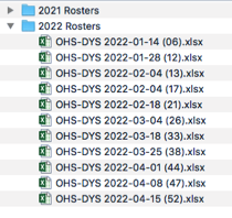

Open the file which is password protected using the PW: gelovitz1. You will enter this twice. Move the window to the side of the screen leaving access to the five files to the left on your desktop.
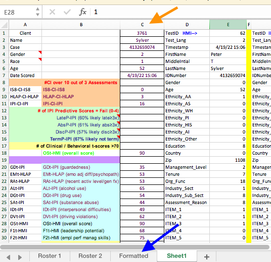
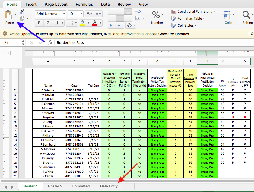
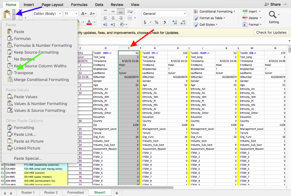
After you opened the Roster, you should see the following spreadsheet. Note the paste button to the left corner (blue arrow) as we’ll use that soon. Also note there are four worksheets in this Excel spreadsheet. You are looking at the first page below. The fourth page is indicated by the red arrow, and this is where you’ll enter the data from the CSV files, so click on the Date Entry button.
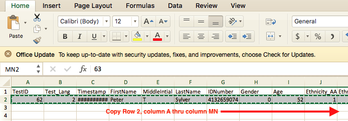
The Data Entry page looks like the following. Assuming you still have the HMI.csv file open on your computer and you have selected all the values in row 2 (see the image above) and copied them (i.e., put the values into memory on the clipboard) now you are ready to paste the values into the Data Entry page.
1. Click on the top of the HMI score entry column (E, red arrow) to select the entire column.
2. Click on the Paste Special button (blue arrow) and then select Transpose.
The values you copied from the HMI.csv file were horizontal (in a row) so you must transpose them into a vertical column, hence you need a “special paste.” Now you can close the HMI.csv file – you’ll see a message asking if you want to save the large amount of data you put on the clipboard, select “no.” [Note if you close it before you do the Transpose Paste, the Special Paste button will be disabled]
OK, now open the IPI.csv file (not the .pdf), copy all the values in row two. Do this by deleting the value in column A, row 2 while holding down the shift key. Then scroll way over the the right until the data ends in field OA and click on that field’s data. Now you’ve selected the entire row of data, just copy it to the clipboard and go to the Roster and select column H, hit special paste and transpose the data into that column. Now you can close the IPI.csv file and don’t save the data. Do the same with the HLAP and IS8 CSV files copying and special pasting into the Roster’s columns.
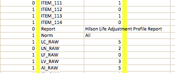
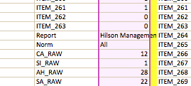
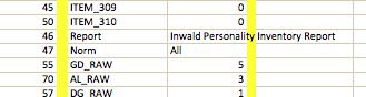
We’re almost done, but now we have to check that the values from the four CSV files transposed correctly (without shifting up or down) into the Roster. Do this by scrolling down the worksheet and making sure the name of each report (green arrow) matches the same rows as column labels (blue arrow). If they don’t line up, you have the wrong data in
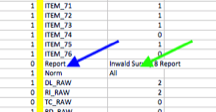
Here’s the other three CSV files showing the report names to the right of the name, each in the proper row.
While you were transposing data into columns E, H, K and N the Excel spreadsheet was calling standardized scores on various scales (see the labels in column B). These scores are all configured in column D (orange arrow). We now need to copy the data in column D into the Formatted worksheet to work on it a bit more.
Simply select the data in column D from row 1 through row 105 and copy it to the clipboard. Then open the “Formatted” worksheet (blue arrow) and go to the next section.